scMultiMap for disease-control studies
Chang Su
2025-06-12
disease_control.RmdThis vignette demonstrates the application of scMultiMap
to infer differentially associated peak-gene pairs using single-cell
multimodal data from disease-control studies.
library(scMultiMap)
library(Signac)
library(Seurat)
# for loading differentially expressed genes
library(openxlsx)
# for making heatmaps
library(ggplot2)
library(pheatmap)
library(RColorBrewer)
In scMultiMap’s manuscript, we applied a permutation procedure to identify significantly differentially associated peak-gene pairs between microglia from healthy control subjects and subjects with Alzheimer’s disease (Results section “scMultiMap mapped GWAS variants of Alzheimer’s disease to target genes in microglia”). We illustrate the codes for this analysis here. At the end of this vignette, we will generate Figures 4b from the manuscript.
Load pre-processed data
We downloaded the single-cell Multiome data on brain from an
Alzheimer’s disease study Anderson et
al., which is the same dataset we used in the manuscript (GSE214979).
We further re-called peaks by cell types with MACS2 using the codes at
the scMultiMap
reproducibility Github repo. Calling peaks by cell types generates
cell-type-specific peaks that better represent candidate
cell-type-specific enhancers than those identified with all cell types
merged, which may obscure signals from less abundant cell types such as
microglia. Using MACS2 provides the fragment counts required for running
scMultiMap.
# set it to the directory where data are saved
data_dir <- '../../../data'

# load AD Multiome data
obj <- readRDS(sprintf('%s/processed_AD_DLPFC_15.rds', data_dir))
# subset to microglia
ct <- 'Microglia'
ct_obj <- subset(x = obj, subset = predicted.id == ct)
In this analysis, we study the top 5000 highly expressed genes and top 50000 highly accessible peaks in microglia, and use a cis-region of width 1Mb to define candidate peak-gene pairs.
pairs_df <- get_top_peak_gene_pairs(subset(x = ct_obj, subset = Diagnosis == 'Unaffected'),
                                    gene_top=5000, peak_top=50000,
                                    distance = 5e+5,
                                    gene_assay = 'RNA', # name of the gene assay
                                    peak_assay = 'peaks') # name of the peak assay
# In the paper, we used control microglia to define peak-gene pairs. (`ct_control`)
# One can also use all microglia.
Here, we generated 135401 candidate peak-gene pairs based on the criterion above. The users can also customize the peak-gene pairs based on your analysis goal.
Differential association analysis
Next, we estimate peak-gene associations in microglia from the
control and the Alzheimer’s disease groups, respectively. Note that
there are multiple biological samples in each group, so
scMultiMap should be run with bsample to avoid
spurious associations due to heterogeneity across biological samples
(see Methods in scMultiMap’s manuscript
for more details).
# multiple biological samples
table(ct_obj$id)
#>
#>     1224     1230     1238     3329     3586     4305     4313     4443
#>      201      161      283      211      152      347       17      171
#>     4481     4482     4627 HCT17HEX   HCTZZT   NT1261   NT1271
#>      233      415      241      264       26      192      265
# control
control_res <- scMultiMap(subset(x = ct_obj, subset = Diagnosis == 'Unaffected'),
                          pairs_df,
                          bsample = 'id', # labels for biological samples in the Seurat object
                          gene_assay = 'RNA', # name of the gene assay
                          peak_assay = 'peaks') # name of the peak assay
#> Start step 1: IRLS
#> Start IRLS for RNA
#> Start IRLS for peaks
#> Start step 2: WLS
#> There are 4652 unique genes in the peak-gene pairs.
#> Warning in sqrt(deno): NaNs produced
#> scMultiMap elapsed time: 01:11 (mm:ss)

# disease
disease_res <- scMultiMap(subset(x = ct_obj, subset = Diagnosis == "Alzheimer's"),
                          pairs_df,
                          bsample = 'id',
                          gene_assay = 'RNA',
                          peak_assay = 'peaks')
#> Start step 1: IRLS
#> Start IRLS for RNA
#> Start IRLS for peaks
#> Start step 2: WLS
#> There are 4652 unique genes in the peak-gene pairs.
#> scMultiMap elapsed time: 01:15 (mm:ss)
The difference between two estimates (the ‘observed difference’) represents the magnitude of differential association. To assess statistical significance, we use a permutation test that randomly reassigns sample labels to disease and control groups 100 times, generating a null distribution of the difference between groups (the ‘null difference’).
# obtain the status for each id (sample)
Status_id_tab <- table(ct_obj$id, ct_obj$Status)
Status_id_tab
#>
#>             AD Ctrl
#>   1224       0  201
#>   1230       0  161
#>   1238       0  283
#>   3329     211    0
#>   3586       0  152
#>   4305     347    0
#>   4313      17    0
#>   4443     171    0
#>   4481     233    0
#>   4482     415    0
#>   4627     241    0
#>   HCT17HEX   0  264
#>   HCTZZT     0   26
#>   NT1261     0  192
#>   NT1271     0  265
Status_ids <- lapply(1:2, function(i) rownames(Status_id_tab)[Status_id_tab[,i] > 0])

all_comb <- combn(rownames(Status_id_tab), length(Status_ids[[1]]))
set.seed(2024)
n_permu <- 100
# randomly reassign 7 samples to the AD group
random_combs <- sample(1:ncol(all_comb), n_permu, replace = F)
We then generated a permutation p-value by evaluating the proportion of times that the “observed difference” is larger in magnitude than the “null difference”.
diff_mat <- matrix(nrow = nrow(control_res), ncol = n_permu)
for(i_permu in 1:n_permu){
  # obtain randomly shuffled sample labels
  disease_sams <- all_comb[,random_combs[i_permu]]
  control_sams <- rownames(Status_id_tab)[!rownames(Status_id_tab) %in% disease_sams]
  # control
  null_control <- scMultiMap(subset(x = ct_obj, subset = id %in% control_sams),
                             pairs_df,
                             bsample = 'id',
                             gene_assay = 'RNA',
                             peak_assay = 'peaks')

  # disease
  null_disease <- scMultiMap(subset(x = ct_obj, subset = id %in% disease_sams),
                             pairs_df,
                             bsample = 'id',
                             gene_assay = 'RNA',
                             peak_assay = 'peaks')

  # null difference, i_permu
  diff_mat[,i_permu] <- null_disease[,'covar'] - null_control[,'covar']
  message(i_permu)
}
obs_diff <- disease_res[,'covar'] - control_res[,'covar']
pval1 <- rowMeans(obs_diff > diff_mat)
pval2 <- rowMeans(obs_diff < diff_mat)
permu_pval <- pmin(pval1, pval2) * 2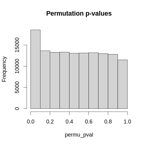
Downstream analysis of differentially associated peak-gene pairs
Enrichment of differentially expressed genes
We assess if genes with differential association are enriched for differential expression.
# microglia DEG from Supplementary table 9 of https://www.nature.com/articles/s41586-024-07606-7
DEG <- read.table(sprintf('%s/aggregated_fullset.Mic_Immune_Mic.tsv.gz', data_dir), header = T)
DEG <- DEG[DEG$region == 'PFC',]
DEG <- DEG[DEG$log10p_nm > -log10(0.05/nrow(DEG)),]
DEG_inds <- control_res$gene %in% DEG$gene

# evaluate enrichment of differentially expressed genes among genes from differentially associated peak-gene pairs
total_gene <- unique(control_res$gene)
DEG_gene <- unique(control_res$gene[DEG_inds])
sig_gene <- unique(control_res$gene[permu_pval < 0.05]) # genes in differentially associated peak-gene pairs (p-value < 0.05)
tab1 <- table(total_gene %in% DEG_gene, total_gene %in% sig_gene)
fisher.test(tab1, alternative = 'greater')
#>
#>  Fisher's Exact Test for Count Data
#>
#> data:  tab1
#> p-value = 6.035e-06
#> alternative hypothesis: true odds ratio is greater than 1
#> 95 percent confidence interval:
#>  1.308737      Inf
#> sample estimates:
#> odds ratio
#>   1.556541
# another set of microglia DEG from supplementary table of https://pmc.ncbi.nlm.nih.gov/articles/PMC10025452/
# wget https://ars.els-cdn.com/content/image/1-s2.0-S2666979X23000198-mmc4.xls
DEG <- read.xlsx(sprintf('%s/1-s2.0-S2666979X23000198-mmc4.xlsx', data_dir), sheet = 'TableS3_ADCtrl_DEGs')
DEG_inds <- control_res$gene %in% DEG$gene[DEG$celltype == 'Microglia']

# evaluate enrichment of differentially expressed genes among genes from differentially associated peak-gene pairs
total_gene <- unique(control_res$gene)
DEG_gene <- unique(control_res$gene[DEG_inds])
sig_gene <- unique(control_res$gene[permu_pval < 0.05]) # genes in differentially associated peak-gene pairs (p-value < 0.05)
tab2 <- table(total_gene %in% DEG_gene, total_gene %in% sig_gene)
fisher.test(tab2, alternative = 'greater')
#>
#>  Fisher's Exact Test for Count Data
#>
#> data:  tab2
#> p-value = 0.01361
#> alternative hypothesis: true odds ratio is greater than 1
#> 95 percent confidence interval:
#>  1.097925      Inf
#> sample estimates:
#> odds ratio
#>   1.482689
Comparing with AD DEGs results from Mathys et al. and Anderson et al., the genes with differential assocations with peaks in microglia are significantly enriched for microglia DEGs with odds ratio 1.56 and 1.48, respectively.
Visualization
We then visualize the associations in control versus disease groups. We focus on peak-gene pairs that (1) are significantlly differentially associated (nominal p-value < 0.05); (2) are significantlly associated in either control or AD microglia (p-value < 0.05); (3) have a difference of correlation greater than 0.2.
subset_inds <- (permu_pval < 0.05) &
    (control_res$pval < 0.05 | disease_res$pval < 0.05) &
    (abs(control_res$cor - disease_res$cor) > 0.2)
coexp_mat <- cbind(control_res$cor, disease_res$cor)
colnames(coexp_mat) <- c('control', 'AD')
g <- pheatmap(t(coexp_mat[DEG_inds & subset_inds,]),
            col = rev(brewer.pal(11, 'RdBu')),
            cluster_rows = F, cluster_cols = T,
            annotation_names_row = F,
            annotation_names_col = F,
            fontsize_row = 15,          # row label font size
            fontsize_col = 7,          # column label font size
            angle_col = 45, # sample names at an angle
            legend_breaks = seq(-1,1,0.2), #c(-1, 0, 1), # legend customisation
            show_colnames = F, show_rownames = T, # displaying column and row names
            cellheight=50, treeheight_col = 15,
fontsize = 12) 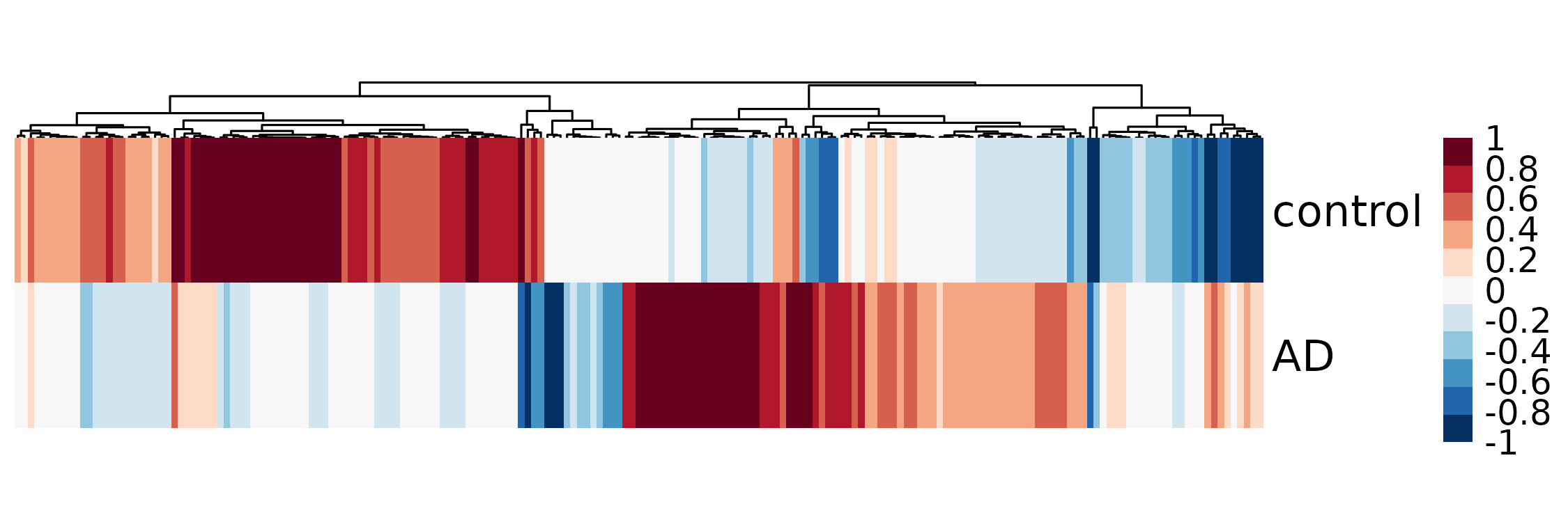
This reproduced Figure~4b in the scMultiMap’s manuscript.
These differentially associated peak-gene pairs can be further analyzed with GWAS (Genome-wide association studies) results, to elucidate the cell-type-specific regulatory mechanisms of GWAS variant in disease relevant cell types. Please see scMultiMap for integrative analysis with GWAS results, a separate vignette that uses differentially associated peak-gene pairs identified here to investigate the function of causal variants of Alzheimer’s disease in microglia.