scMultiMap for integrative analysis with GWAS results

This vignette demonstrates how to apply scMultiMap to map associated peak-gene pairs and integrate the results with genome-wide association studies (GWAS) to elucidate the regulatory functions of GWAS variants in disease-associated cell types. As an example, we will reproduce the results from the scMultiMap manuscript, specifically those presented in the section ‘scMultiMap mapped GWAS variants of Alzheimer’s disease to target genes in microglia.’ At the end of this vignette, we will generate Figures 4d and 4e from the manuscript.

library(scMultiMap)
library(Signac)
library(Seurat)
library(ggplot2)
library(openxlsx)
library(GenomicRanges)

Motivation

Over 75 genetic loci have been associated with the risk of developing Alzheimer’s disease (AD) (Bellenguez, C. et al.), yet their regulatory functions and relevant cellular contexts remain unclear. Among brain cell types, microglia—the brain’s innate immune cells—exhibit the highest enrichment of genetic association with AD in their cis-regulatory elements (Nott, A. et al., Gjoneska, E. et al.). Therefore, this analysis focuses on microglia and uses scMultiMap to identify candidate pairs of cis-regulatory elements and their target genes. As two examples, we examine how scMultiMap results can elucidate the regulatory function of fine-mapped AD variants in microglia at two loci: PICALM and INPP5D.

Run scMultiMap

Note: this vignette use the same dataset as in vignette: scMultiMap for disease-control studies. Please refer to it for details on pre-processing data and running scMultiMap.

# set it to the directory where data are saved
data_dir <- '../../../data' 

# load AD Multiome data
obj <- readRDS(sprintf('%s/processed_AD_DLPFC_15.rds', data_dir))
# subset to microglia
ct <- 'Microglia'
ct_obj <- subset(x = obj, subset = predicted.id == ct)

In this analysis, we study the top 5000 highly expressed genes and top 50000 highly accessible peaks in microglia, and use a cis-region of width 1Mb to define candidate peak-gene pairs.

pairs_df <- get_top_peak_gene_pairs(ct_control,
                                    gene_top=5000, peak_top=50000,
                                    distance = 5e+5,
                                    gene_assay = 'RNA', # name of the gene assay
                                    peak_assay = 'peaks') # name of the peak assay
# In the paper, we used control microglia to define peak-gene pairs. (`ct_control`)
# One can also use all microglia.

Here, we generated 135401 candidate peak-gene pairs based on the criterion above. The users can also customize the peak-gene pairs based on your analysis goal.

Next, we estimate peak-gene associations in microglia from the control and the Alzheimer’s disease groups, respectively. Note that there are multiple biological samples in this dataset, so scMultiMap should be run with bsample to avoid spurious associations due to heterogeneity across biological samples (see Methods in scMultiMap’s manuscript for more details).

# multiple biological samples
table(ct_obj$id)
#> 
#>     1224     1230     1238     3329     3586     4305     4313     4443 
#>      201      161      283      211      152      347       17      171 
#>     4481     4482     4627 HCT17HEX   HCTZZT   NT1261   NT1271 
#>      233      415      241      264       26      192      265

# control
control_res <- scMultiMap(ct_control, 
                          pairs_df,
                          bsample = 'id',
                          gene_assay = 'RNA',
                          peak_assay = 'peaks')
#> Start step 1: IRLS
#> Start IRLS for RNA
#> Start IRLS for peaks
#> Start step 2: WLS
#> There are 4652 unique genes in the peak-gene pairs.
#> Warning in sqrt(deno): NaNs produced
#> scMultiMap elapsed time: 01:13 (mm:ss)

# disease
disease_res <- scMultiMap(ct_AD, 
                          pairs_df,
                          bsample = 'id',
                          gene_assay = 'RNA',
                          peak_assay = 'peaks')
#> Start step 1: IRLS
#> Start IRLS for RNA
#> Start IRLS for peaks
#> Start step 2: WLS
#> There are 4652 unique genes in the peak-gene pairs.
#> scMultiMap elapsed time: 01:16 (mm:ss)

What does “Warning in sqrt(deno): NaNs produced” mean?

This warning suggests that some peaks or genes have variance estimated to be negative, causing numerical errors in calculating correlations. This situation is typically rare and may happen when you consider genes or peaks with extremely low abundance (e.g. top 5000 genes and top 50000 peaks here). The estimated correlations will be internally set to 0 by scMultiMap.

Load results on fine-mapped AD GWAS variants

# AD GWAS variants fine-mapped and priortized based on eQTL & Hi-C
# "Seeding from PAINTOR or FGWAS 95% credible set variants (Sup- plementary Table 6b), 
# we first included their linkage disequilibrium (LD) tags (defined as LD R2 > 0.8) in TOP-LD European (EUR) 
# and then retained only those overlapping microglia ATAC–seq peaks that interact with promoters"
#
# Reference: https://www.nature.com/articles/s41588-023-01506-8
# Data source: supplementary table 6b

mic_fm_prior_variants_df <- read.xlsx(sprintf('%s/41588_2023_1506_MOESM3_ESM.xlsx', data_dir),
                                sheet = 'Supplementary Table 6c', startRow = 2)
mic_fm_prior_variants_df$chr <- paste0('chr', mic_fm_prior_variants_df$chr)
grange_mic_fm_prior <- GenomicRanges::makeGRangesFromDataFrame(df = mic_fm_prior_variants_df, 
                                                         seqnames.field = 'chr',
                                                         start.field = 'pos.hg38',
                                                         end.field = 'pos.hg38')

Visualize inferred peak-gene links and fine-mapped GWAS variants

PICALM locus (figure 4d)

# make grange objects that connect genes with peaks
gene_peak_link_gr_control <- make_gene_to_peak_link(control_res, 'PICALM', ct_control, 'peaks')
gene_peak_link_gr_AD <- make_gene_to_peak_link(disease_res, 'PICALM', ct_AD, 'peaks')
gene_peak_link_list <- list(AD = gene_peak_link_gr_AD, control = gene_peak_link_gr_control)

uniform_fs <- 20
# genomic region around PICALM locus
selected_range <- "chr11-85850000-86216290"

gene_plot <- AnnotationPlot(
  object = ct_control,
  region = selected_range
) + theme(text = element_text(size = uniform_fs)) 

link_plot_list <- list()
for(g in c('control','AD')){
    Links(ct_obj) <- gene_peak_link_list[[g]][abs(gene_peak_link_list[[g]]$score) > 0.2]
    link_plot_list[[g]] <- LinkPlot(
        object = ct_obj,
        region = selected_range
    ) + scale_color_gradient2(low = "blue",
                              midpoint = 0,
                              mid = "white",
                              high = "red",
                              space="Lab",
                             limits = c(-1,1)) +
    labs(color = 'correlation', y = sprintf('%s', g)) +
    theme(text = element_text(size = uniform_fs))
}
#> Scale for colour is already present.
#> Adding another scale for colour, which will replace the existing scale.
#> Scale for colour is already present.
#> Adding another scale for colour, which will replace the existing scale.

expr_plot <- ExpressionPlot(
  object = ct_obj,
  features = "PICALM",
  assay = "SCT",
    group.by='Status'
)  +
theme(text = element_text(size = uniform_fs))

# to see it on the plot
end(grange_mic_fm_prior) <- end(grange_mic_fm_prior) + 1000

DefaultAssay(ct_obj) <- 'peaks'
snp_plot <- PeakPlot(
  ct_obj,
  selected_range,
  assay = NULL,
  peaks = grange_mic_fm_prior,
  group.by = NULL,
  color = "black",
  sep = c("-", "-")
) + labs(y = 'SNPs') +
    theme(text = element_text(size = uniform_fs))

g <- CombineTracks(plotlist = list(gene_plot, snp_plot, link_plot_list[[1]], link_plot_list[[2]]),
                   expression.plot = expr_plot,
                   heights = c(2,1,2,2) * 5/7,
                   widths = c(6.5, 1))
g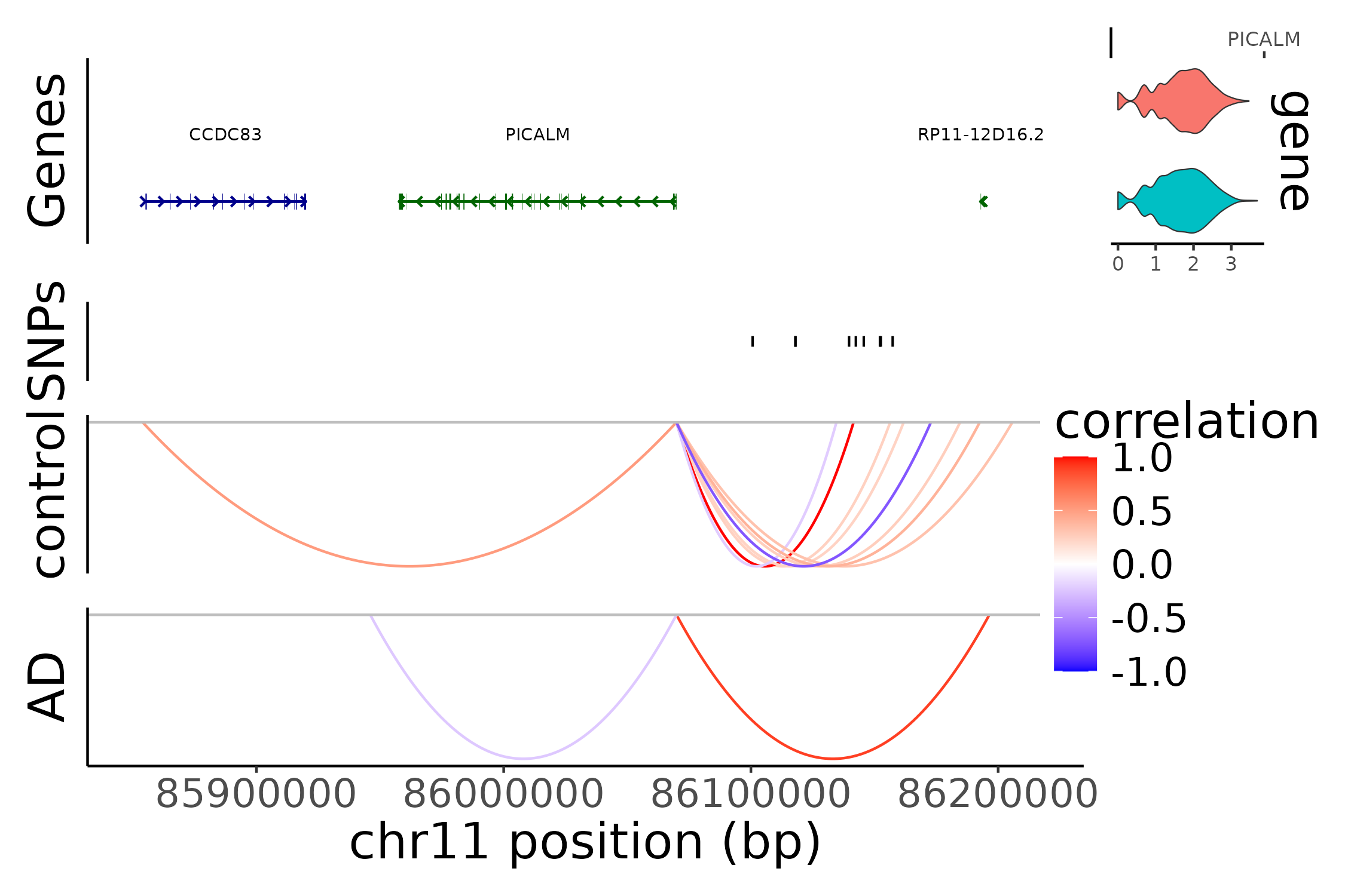

This reproduced Figure~4d in the scMultiMap’s manuscript.

INPP5D locus (figure 4e)

Repeat the analysis above for the INPP5D locus.

# make grange objects that connect genes with peaks
gene_peak_link_gr_control <- make_gene_to_peak_link(control_res, 'INPP5D', ct_control, 'peaks')
gene_peak_link_gr_AD <- make_gene_to_peak_link(disease_res, 'INPP5D', ct_AD, 'peaks')
gene_peak_link_list <- list(AD = gene_peak_link_gr_AD, control = gene_peak_link_gr_control)

uniform_fs <- 20
# genomic region around INPP5D locus
selected_range <- "chr2-232850000-233259353"

gene_plot <- AnnotationPlot(
  object = ct_control,
  region = selected_range
) + theme(text = element_text(size = uniform_fs)) 

link_plot_list <- list()
for(g in c('control','AD')){
    Links(ct_obj) <- gene_peak_link_list[[g]][abs(gene_peak_link_list[[g]]$score) > 0.2]
    link_plot_list[[g]] <- LinkPlot(
        object = ct_obj,
        region = selected_range
    ) + scale_color_gradient2(low = "blue",
                              midpoint = 0,
                              mid = "white",
                              high = "red",
                              space="Lab",
                             limits = c(-1,1)) +
    labs(color = 'correlation', y = sprintf('%s', g)) +
    theme(text = element_text(size = uniform_fs))
}
#> Scale for colour is already present.
#> Adding another scale for colour, which will replace the existing scale.
#> Scale for colour is already present.
#> Adding another scale for colour, which will replace the existing scale.

expr_plot <- ExpressionPlot(
  object = ct_obj,
  features = "INPP5D",
  assay = "SCT",
    group.by='Status'
)  +
theme(text = element_text(size = uniform_fs))

# to see it on the plot
end(grange_mic_fm_prior) <- end(grange_mic_fm_prior) + 1000

DefaultAssay(ct_obj) <- 'peaks'
snp_plot <- PeakPlot(
  ct_obj,
  selected_range,
  assay = NULL,
  peaks = grange_mic_fm_prior,
  group.by = NULL,
  color = "black",
  sep = c("-", "-")
) + labs(y = 'SNPs') +
    theme(text = element_text(size = uniform_fs))

g <- CombineTracks(plotlist = list(gene_plot, snp_plot, link_plot_list[[1]], link_plot_list[[2]]),
                   expression.plot = expr_plot,
                   heights = c(2,1,2,2) * 5/7,
                   widths = c(6.5, 1))
g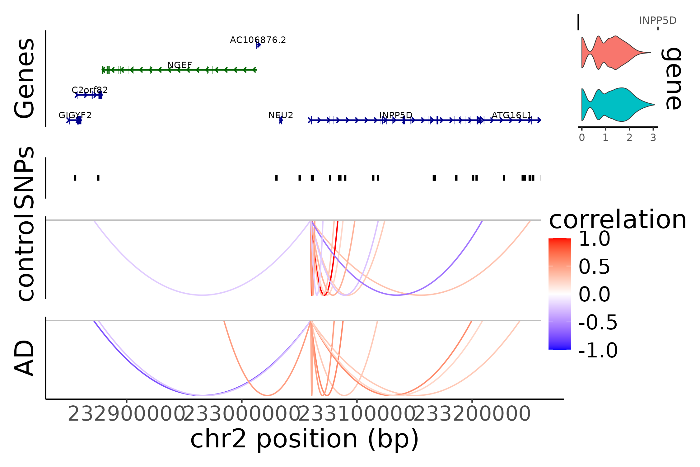

This reproduced Figure~4e in the scMultiMap’s manuscript.